What is Big O Notation? Why it is Important For Coding Interviews?

Big O notation is a mathematical notation that describes the limiting behavior of a function when the argument tends towards a particular value or infinity.

Big O notation is a mathematical notation that describes the limiting behavior of a function when the argument tends towards a particular value or infinity.

This sounds scary and intimidating to a lot of engineers and they tend to skip this important topic and lean towards solving coding problems.

So, generally what is a Big O then? We use Big O to describe the performance of an algorithm. This helps to determine if a given algorithm is scalable or not.

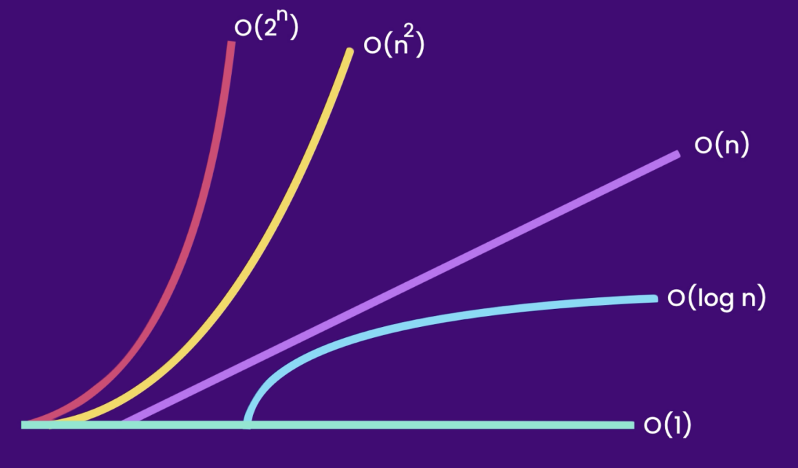
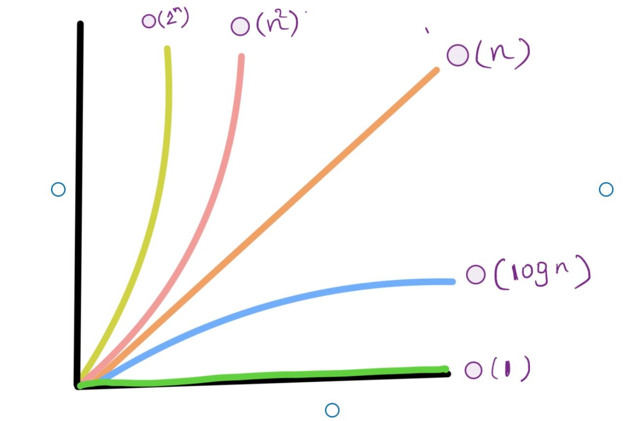
Let us see a graph that will help you understand the time complexities which are available in computer science.

Scalable means if an algorithm scales when input grows large. Just because your computer executes the code doesn’t mean it is scalable.

This is the reason we use Big O notation to describe the performance of an algorithm. Well, what does this has to do with data structures?

Let us see an Array example to understand this.

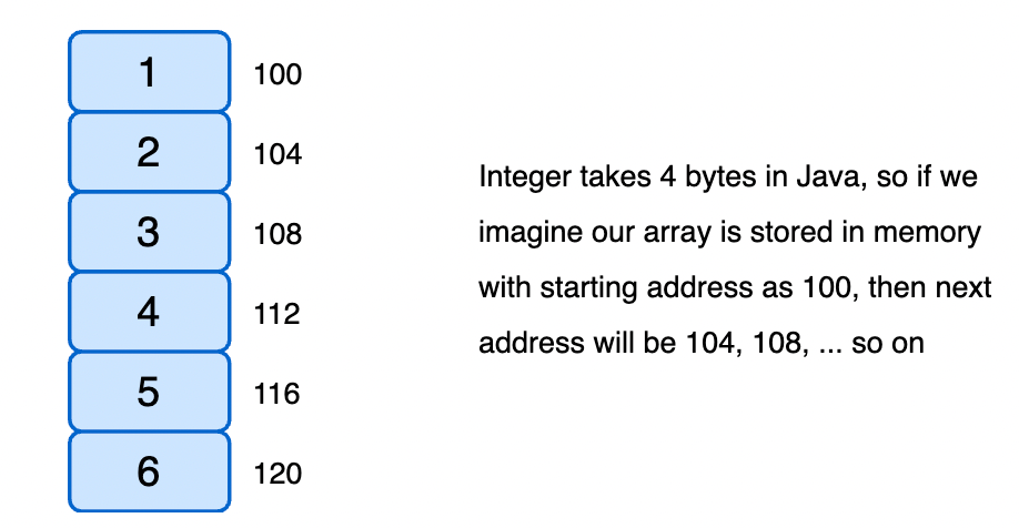
In the above example, array[0] prints 1 on the console.

But arrays are fixed size, so if we have to add or remove items then it becomes expensive as we need to increase or decrease the original array.

What if an array grows and has millions of items in it?

It’s obviously an even more expensive operation when adding elements at the middle or removing an element at the start. This is because we have to shift the entire array based on insertion or deletion.

This is where LinkedList comes into the picture. LinkedList can grow and shrink quickly, but accessing a linked list element is expensive as we need to traverse the whole linked list which is O(n).

This is the reason we need to learn the big-O first before we start data structures.

Note:  Top tech companies like FAANG ( Facebook, Amazon, Apple, Netflix, and Google ) always talk about Big-O, just to understand how scalable the algorithm you have written is!

Finally knowing Big-O will make you a better and good software engineer.

So over time we start with Data Structures and work on the Big-O of all of them. Let us learn more about the various time complexities we have in computer science.

1. Constant Time Complexity – O(1).
2. Linear Time Complexity – O(n).
3. Quadratic Time Complexity – O(n^2).
4. Logarithmic Time Complexity – log(n).
5. Exponential Time Complexity – O(2^n).

1. Constant Time Complexity: O(1)

Let us run through an example and talk more about the constant time complexity. Here is the simple snippet explaining the O(1) time.

ContantTime Code:-

public class ConstantTime {
  public static void main(String[] args) {
    int[] numbers = {1, 2, 3, 4, 5};
    constantTime(numbers);
  }

  // Overall, O(1) constant time
  private static void constantTime(int[] numbers) {
    System.out.println(numbers[0]); // O(1)
    System.out.println(numbers[1]); // O(1)
    System.out.println(numbers[4]); // O(1)
  }
}

In the above snippet, we are printing array elements by index, and it’s super fast since we are accessing it through index-based.

In the above example if we have to iterate over the elements to find an element from the array then the time complexity takes O(n), as in the worst-case scenario, we find the element at the last index of the array.

2. Linear Time Complexity – O(n)

Here is the classic example where we iterate through all the elements and print each item on the console. This is where the size of input varies.

This is not worse compared to the logarithmic and constant time complexities.

So,

1. If we have 5 items, we print 5 console items.
2. If we have a million items, we print a million entries on the console.

So, this grows as the input grows linearly, which means it is directly proportional to the input size.

What if we were asked to find an element from an array of integers, on the worst-case scenario we find this at the last index. This means our loop is run over the loop starting from the first index until last and the time it takes is O(n).

So the run time complexity is O(n), where n is the size of the array. Here is an example snippet explaining the linear time complexity.

LinearTime Code:-

public class LinearTime {
  public static void main(String[] args) {
    int[] numbers = {1, 2, 3, 4, 5};
    linearTime(numbers);
  }

  // O(n) linear time
  private static void linearTime(int[] numbers) {
    for (int number : numbers) { // O(n)
      System.out.println(number); // O(1)
    }
  }
}

So the cost of the algorithm is dependent on the size of the input. No matter, we replace this with any other advanced pre-defined methods, the time complexity is always O(n). Let us replace this with the forEach loop.

public class LinearTime {
  public static void main(String[] args) {
    int[] numbers = {1, 2, 3, 4, 5};
    linearTimeForEach(numbers);
  }

  // O(n) linear time
  private static void linearTimeForEach(int[] numbers) {
    System.out.println("Items are: "); // O(1)
    for (int number : numbers) { // O(n)
      System.out.println(number);
    }
    System.out.println("end line ---"); // O(1)
  }
}

From the above snippet, we can see the run time is O(1) + O(n) + O(1), which is O(n), we drop the constants, when we have a bigger complex runtime. Hence the time complexity for this is O(n).

Let us see another example below.

public class LinearTime {
  public static void main(String[] args) {
    int[] numbers = {1, 2, 3, 4, 5};
    linearTimeForEach(numbers);
  }

  // O(n) linear time
  private static void linearTimeForEach(int[] numbers) {
    System.out.println("Items are: "); // O(1)
    for (int number : numbers) { // O(n)
      System.out.println(number);
    }

    for (int number : numbers) { // O(n)
      System.out.println(number * number);
    }
    System.out.println("end line ---"); // O(1)
  }
}

What if we have two for-loops one after another. So overall the time complexity is O(n) + O(n) => 2*O(n)=> O(n).

We drop the constant and now, the approximation of the algorithm cost is proportional to the size of the input. O(n) still represents the linear time complexity.

Let us see another example with different inputs.

public class LinearTime {
  public static void main(String[] args) {
    int[] numbers = {1, 2, 3, 4, 5};
    String[] movies = {"The Shawshank Redemption", "Taxi Driver", "Schindler's List", "The Princess Bride"};
    linearTimeForEach(numbers, movies);
  }

  // O(n) linear time
  private static void linearTimeForEach(int[] numbers, String[] movies) {
    for (int number : numbers) { // O(n)
      System.out.println(number);
    }

    System.out.println("---------");

    for (String movie : movies) { // O(m)
      System.out.println(movie);
    }
  }
}

In the above example, we have two for-loops running on two different inputs.

So, the time complexity is O(n + m). Where n is the size of the numbers array and m is the size of the string array

We cannot ignore either of the n or m sizes of arrays.

3. Quadratic Time Complexity - O(n^2)

Quadratic time complexity is not often recommended as time complexity is directly proportional to two times the size of the input. Let us see an example below.

public class QuadraticTime {
  public static void main(String[] args) {
    int[] numbers = {1, 2, 3, 4, 5};
    quadraticTime(numbers);
  }

  private static void quadraticTime(int[] numbers) {
    // overall O(n * n) or O(n^2) time complexity
    for (int firstNumber : numbers) { // O(n) tim
      for (int secondNumber : numbers) { // O(n) time
        System.out.println(firstNumber + " " + secondNumber);
      }
    }
  }
}

So overall the time complexity is O(n^2).

As for each indexed element we run across the entire array and we print them.

So if an array has 5 elements, then the second loop runs for every element in the array. 5*5 is 25 times the loop runs. If the array contains a million items in it, then the loop runs a (million * million).

Note: Imagine if we have a nested(quadratic) loop running and another linear time loop. Then the overall time complexity will be O(n)+O(n^2), which is equivalent to O(n^2). Since we drop the linear time as the quadratic one is larger than the linear. So, if a nested loop has three inner loops then the time complexity is O(n^3).

4. Logarithmic Time Complexity - log(n)

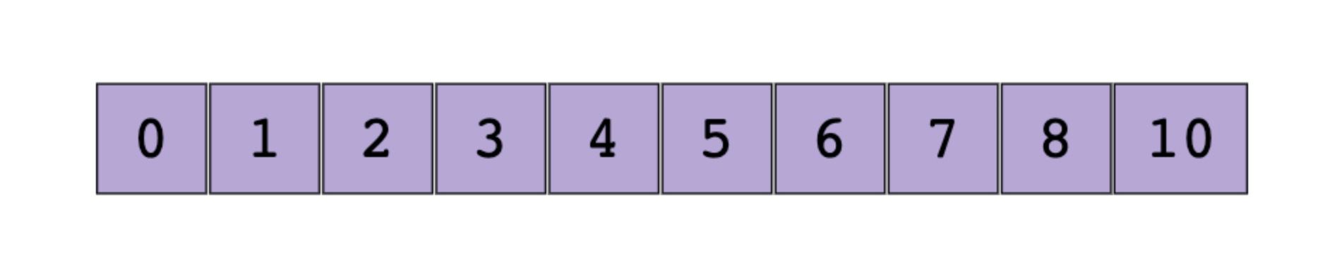
Logarithmic time complexity is better than linear time. So an algorithm running at logarithmic is more efficient and more scalable than a linear one. Let us imagine that we have an array of sorted integers from 1 over 10.

We can iterate over all the elements, which is called linear search.

In this, we run through each element present in the array using an index and the time complexity is always O(n), which is linear time. But, is there a better way to solve this problem? Yes, we can use an optimal way by dividing the halves of an array by searching the element in the array, which is called a Binary search algorithm.

A binary search algorithm divides the array into halve each time and find the element fastly. In the above example, if we have to find element 10 then we first divide the array into halve, and then we check the middle element is equal or not and we do it over until we find the result.

Here is the snippet that does this and we only run the loop 4 times and find the element we were looking for. Here is the snippet below explaining it.

public class BinarySearch {
  public static void main(String[] args) {
    int[] array = {1, 2, 3, 4, 5, 6, 7, 8, 9, 10};
    System.out.println("Element found at index "+binarySearch(array));
  }

  private static int binarySearch(int[] array) {
    int left = 0, right = array.length - 1, middle = -1;

    while (left <= right) {
      System.out.println("Running...");
      middle = (left + right) / 2;
      if (array[middle] == 10) {
        return middle;
      } else if (array[middle] < 10) {
        left = middle + 1;
      } else if (array[middle] > 10) {
        right = middle - 1;
      }
    }
    return middle;
  }
}

// Prints following on the console
Running...
Running...
Running...
Running...
Element found at index 9

So for each loop, we are dividing the array elements into half and hence the time complexity is always logarithmic or log(n).

5. Exponential Time Complexity - O(2^n)

An algorithm running exponential time is not scalable. As this becomes much slower and the algorithm runs much slower this algorithm is never appreciated at all.